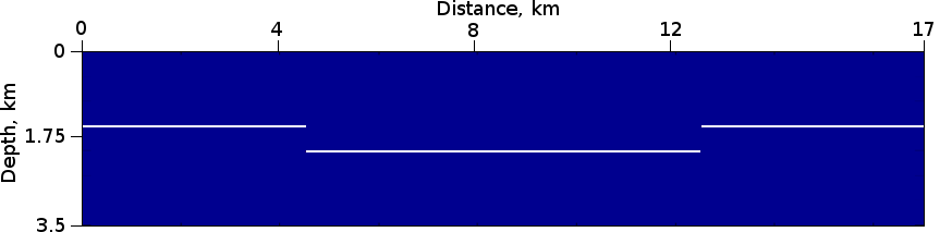
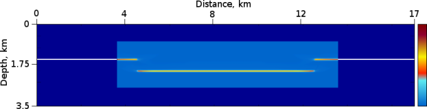
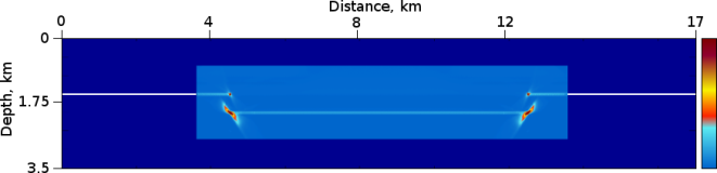
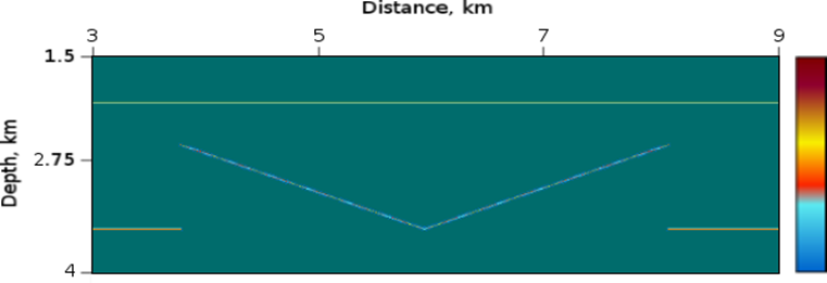
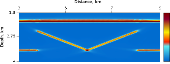
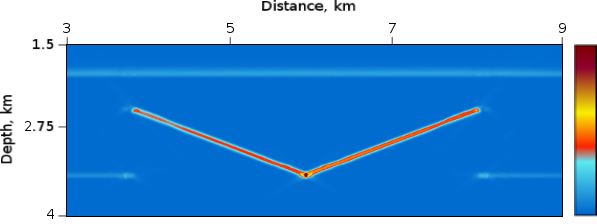
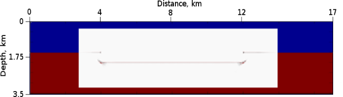
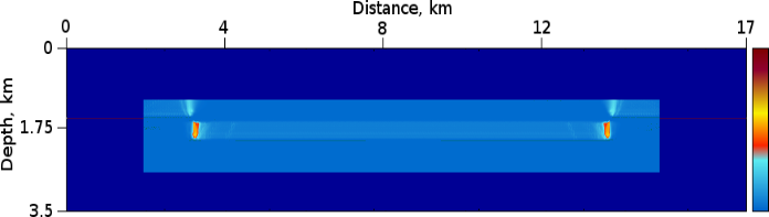
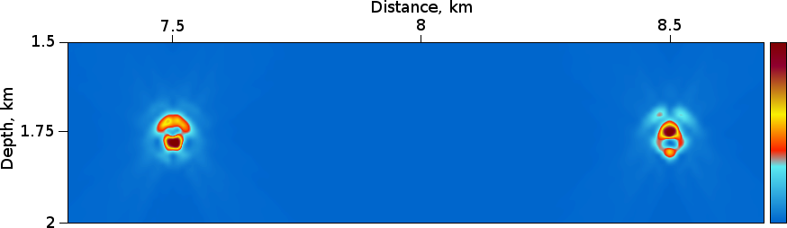
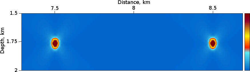
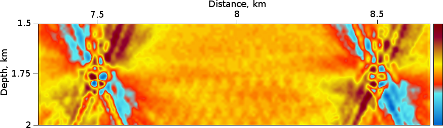
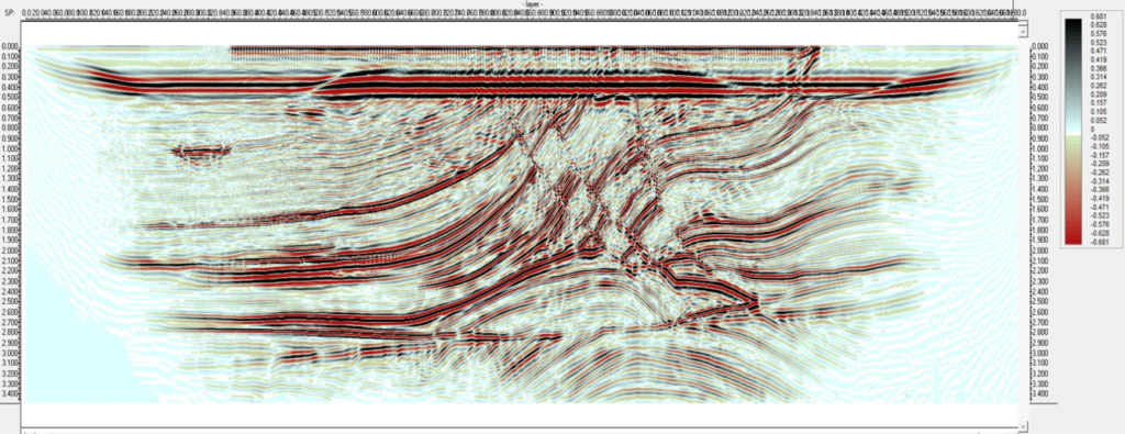
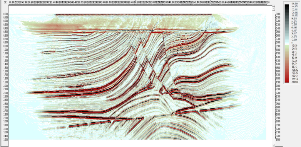
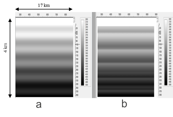
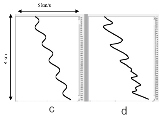
Figure 2 : RTH Depth Migration soft diffractor filter (a), hard diffractor filter (b), soft & hard diffractor filter (c), RTH Dip Angle Variance (d).
More detail:
Erokhin G., Pestov L., Danilin A., Kozlov M., and Ponomarenko D., 2017,
Interconnected vector pairs image conditions: New possibilities for visualization of acoustical media, 2017, SEG Technical Program Expanded Abstracts 2017: 4624-4629., https://doi.org/10.1190/segam2017-17587902.1
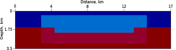
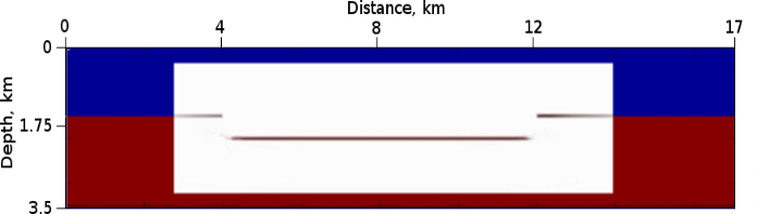
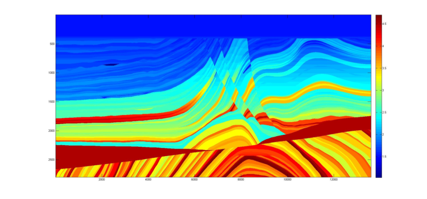
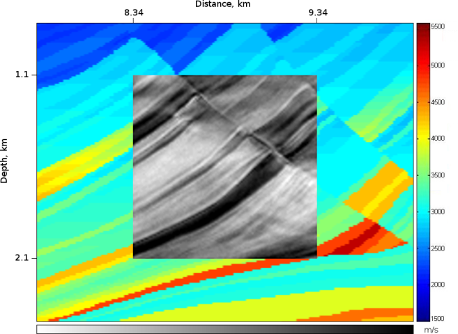
Marmousei2 model.